A super important function in dataanalysis is joining two or more tables, socalled table - join in Data Science limbo. Many of us work with SAP as a data source for their analysis. This data source is well known for being based on a large number of tables (> 100.000). Other ERP systems also store the enterprise data in relational tables, which means in several tables. Therefore, for a data analyst it is essential to be able to link several, individual tables into one.
That's what IDEA can do. Best of all, you don´t need any programming skills for that. Just the program and you. Because the feature is so important, here's comes the quick guide for joining tables:
IDEA features two functions for table joins. Since this is a quick guide, in this post I'll show you the simpler and faster version of the visual connection. In a separate post you will find a description of a more extensive tables join function.
The advantage of the visual linking in IDEA is that you can join multiple tables in one instance. For the beginning, however, two are enough:

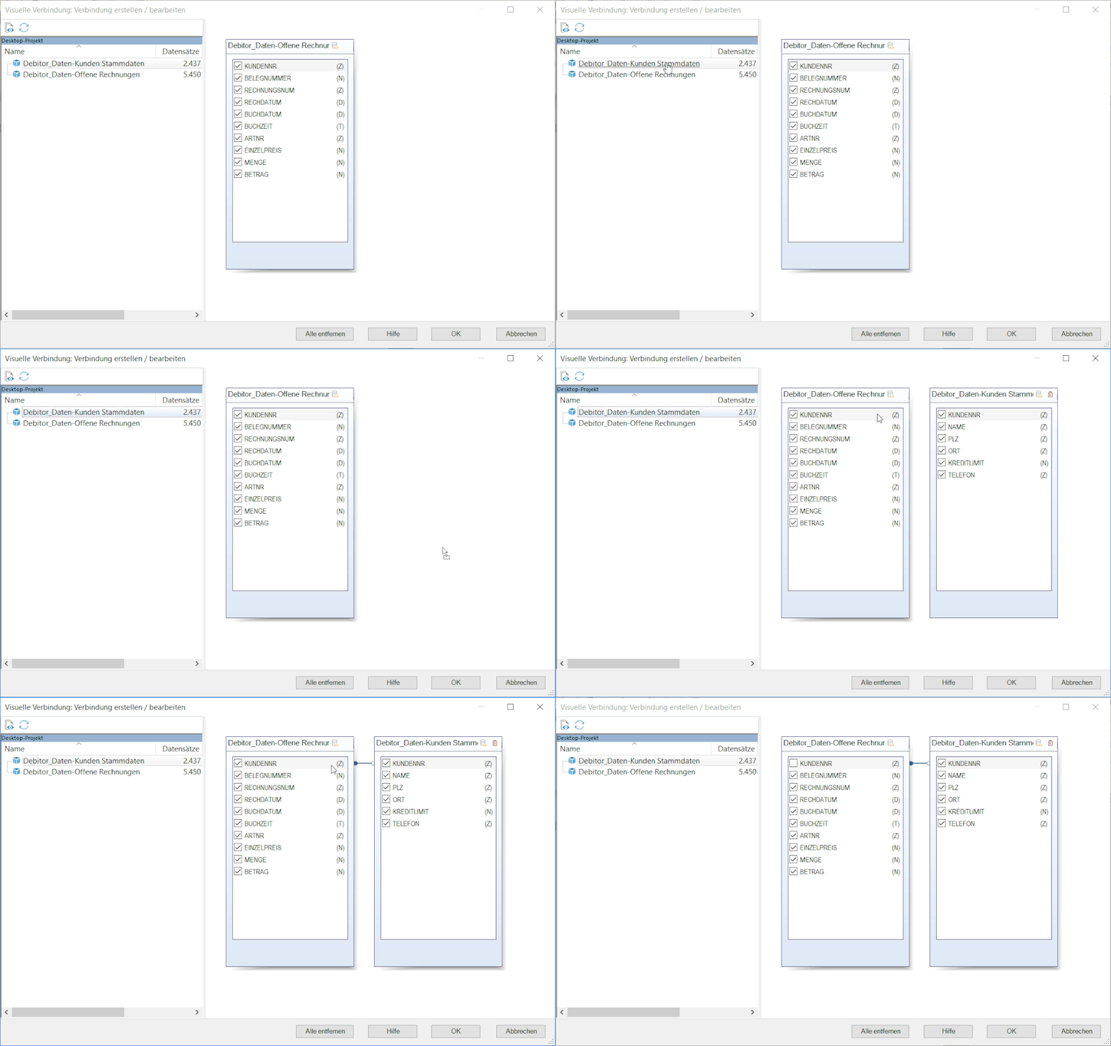
So, with the first table already opened, you click the tab "Analysis" and -surprise, surprise- "Visual Connector" (You find it in the group called “Relate”).
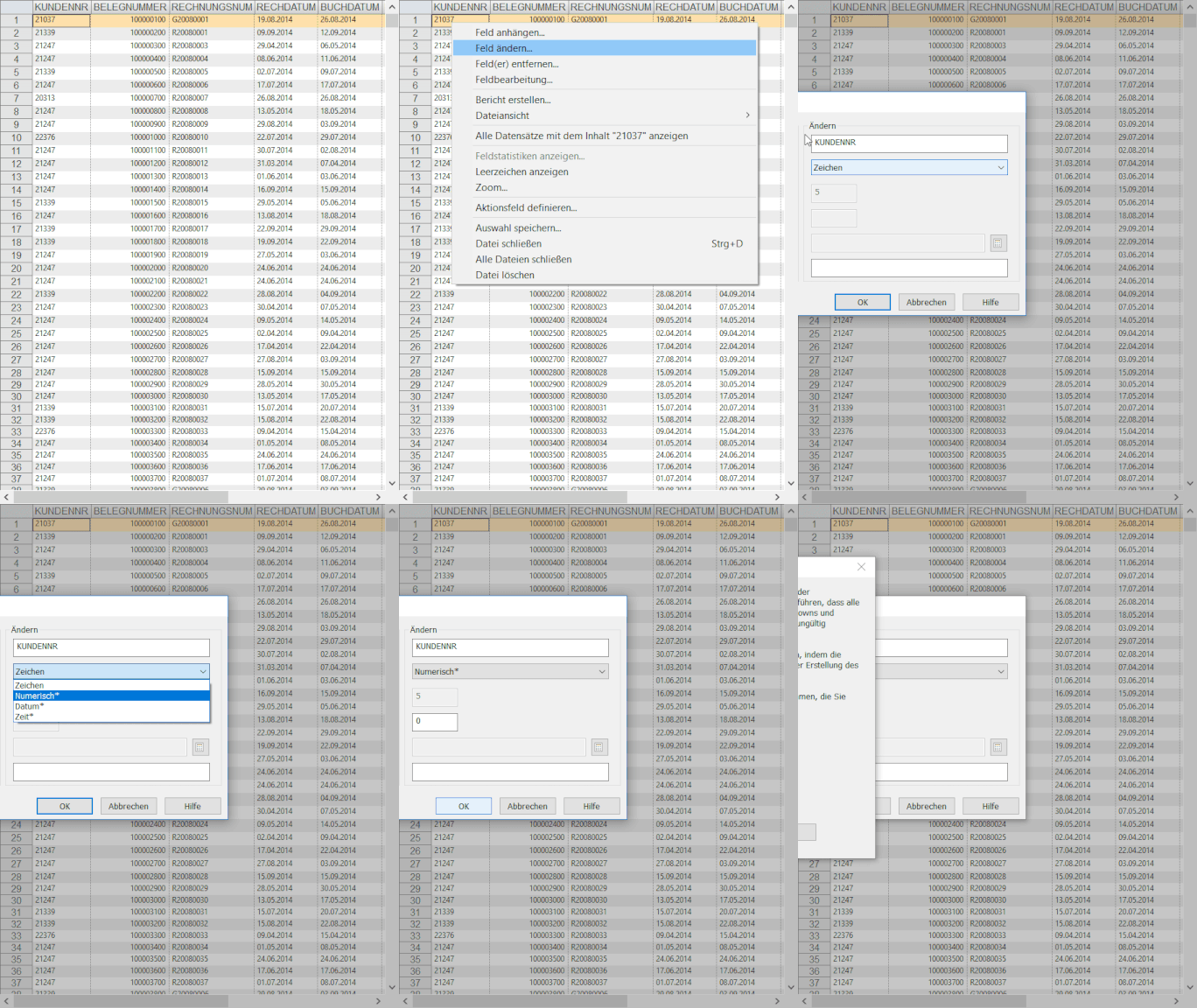
Within the new window then open the second table by double-clicking on it. Now we have both tables and their column names clearly arranged side by side in the visual area on the right side. Next to the column names you can see the character or field type ("N" for numeric and "C" for Character). It is important to ensure that only the same character types, that means only N with N and Z only with Z, can be connected to each other.

What does not fit is made to fit (as we say in Germany sometimes)!
So, in the case character types do not match, we'll match them. Click on one of the tables with a right mouse click on the corresponding column and then select "change field". Here you change the appropriate field types. You can or better should answer the following warning message with "yes" and as a result you already matched the field types. The GIF displays these steps --}
In general, when connecting or joining tables, the goal is to find the common identifier or match key or key index in both tables in order to attach the appropriate line of the second file to its corresponding line of the primary file. In the example shown here, we attach the customer master data using the key index "Customer No." from the database "Debitor_Daten - Kunden Stammdaten” to each open invoice from table “Debitor_Daten - Offene Rechnungen” with the same common match key customer number in column “Kundennr”.

Back to our visual connection in IDEA, using drag and drop, we create a visual link between the key indexes of the two tables, as seen beautifully in the GIF. Now IDEA knows how to make two tables one.

What is actually connected now?
Rarely do I have data in the first table that can be 100% linked to a second table. To clarify this issue a bit more in detail, let´s briefly enter the mathematical set theory:

As can be seen in the result of our example, the primary file over the open invoices had 5450 rows; the resulting file including the billing and customer master data, however, only 5443 lines. So, seven rows went overboard. That means, the resulting joined table only includes rows that could be connected via the index key.
And this shows us the disadvantage of the visual connection compared to the “non-visual” join function in IDEA: The visual connection does not allow to determine which which part of the original datasets enter the result database.
IDEA´s full join function of IDEA, however, specifies, for example, whether all rows of the first file or all rows that do not match or or ... get into the result file. A clear advantage of the normal table join with IDEA. So be aware of this difference of the two table join functions!

The clear advantage of the visual connection in IDEA, however, is speed and ease of use. As a good accountant always says, "It depends on what you want."

Kommentar schreiben